

Wireless Communication
 EU RED Network Security Standard EN 18031
 Wireless and communication detection
 Mobile communication product certification
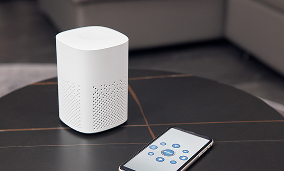 Bluetooth BQB Product Certification
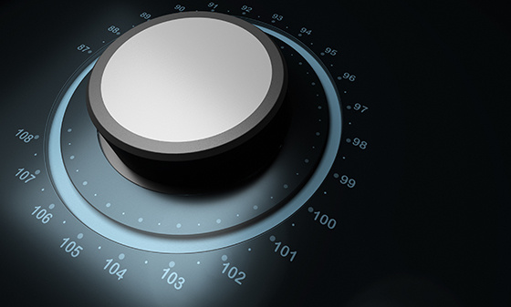 FM/AM Product Certification
 WiFi Product Certification
 Wireless charging product certification
 Interphone product certification
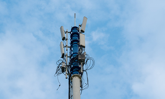 Base station certification
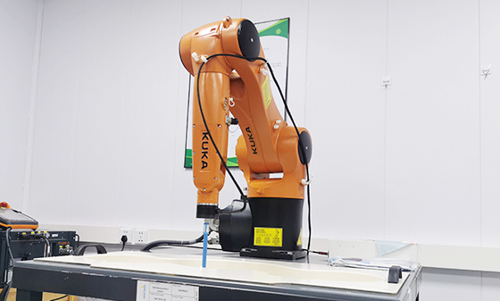 SAR testing
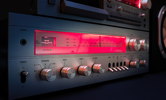 Receiver Product Certification
 5G NR Product Certification
 UWB Product Certification
 Internet of Things authentication
Electromagnetic compatibility
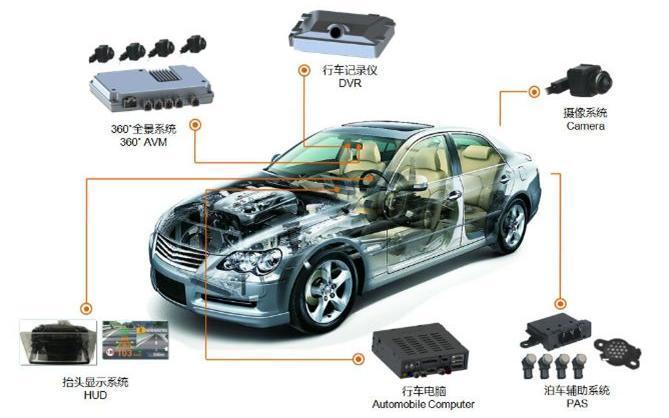 Automotive Electronics EMC Testing
 EMC rectification
 EMC
EMC
Automotive Electronics
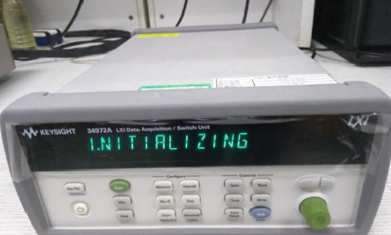 Electrical performance testing
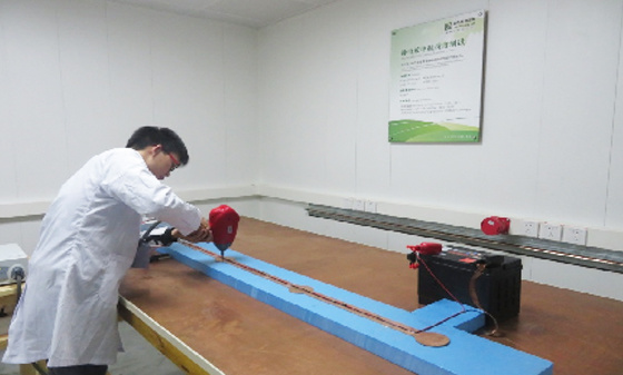 EMS testing - radiation anti-interference testing system (including radar waves)
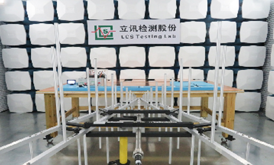 EMS Testing - Electrostatic Discharge
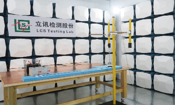 EMS Test - Transient Conducted Immunity Test
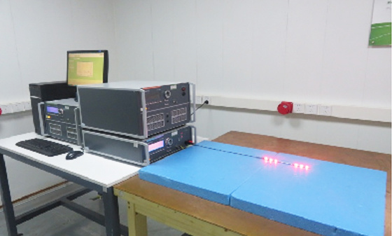 EMS Testing - Portable Transmitter Immunity
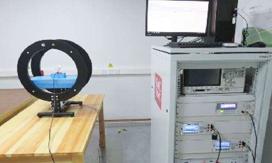 EMS Test - High Current Injection (BCI) Test
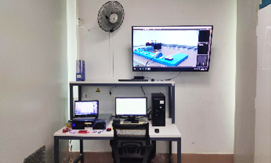 EMS test - low-frequency magnetic field anti-interference test
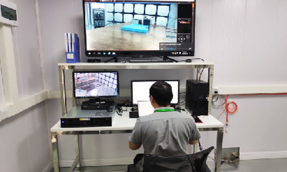 EMI Testing - Transient Conducted Emissions Testing System
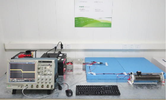 EMI testing - low-frequency magnetic field emission
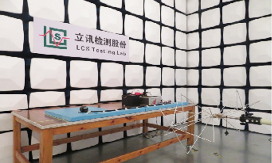 EMI Test - Radiation Emission Test
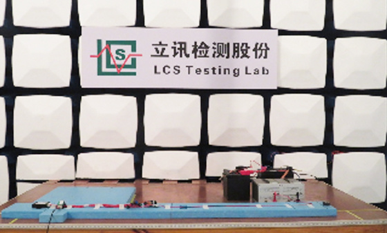 EMI Test - Conducted Emissions Test
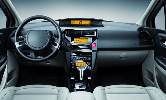 Automotive Electronic Testing
Automotive Parts Inspection
 Automotive ELV&VOC
 Reliability testing
 Temperature shock test
 Vibration testing
 Instrument panel/instrument panel three comprehensive vibration test
 Comprehensive vibration test of door inner panel III
 Sunvisor Three Comprehensive Vibration Test
 Spoiler Three Comprehensive Vibration Test
 Three comprehensive vibration tests of car front and rear bumpers
 Three comprehensive vibration tests for lamp housing/lampshade
 Comprehensive vibration test of outer circumference three
 Automotive metal material testing
 Performance testing of automotive lighting fixtures
 Rapid temperature change test
 Vibration
 Common issues with vibration testing
 Common issues with fatigue testing
 Common issues with high and low temperature testing
 Conducted Interference (CE) - Suzhou Lixun Standard
 Electromagnetic Radiation Tolerance Test (RS) - Suzhou LCS Standard
 Electrical Fast Pulse Withstand Test (EFT) - Suzhou LCS Standard
 Voltage flicker test - Suzhou LCS standard
Electronic appliances
 Household appliance product testing
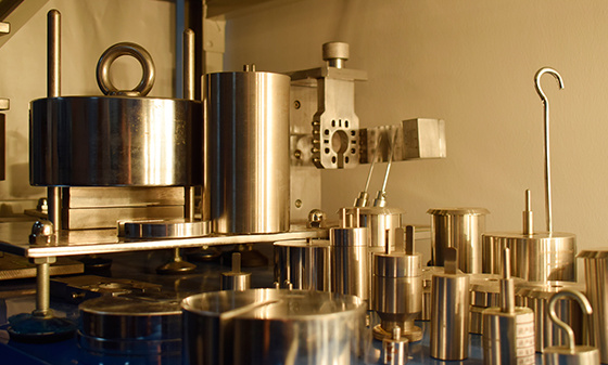 Electrical accessory product testing
 Household appliance testing
Chemical Testing
 Introduction to PFAS Testing
 MOSH/MOAH Mineral Oil Testing Service
 MOSH/MOAH Mineral Oil Testing and Certification Report Service
 Consumer Product Testing Services - WEEE Chapter
 Ecological textile testing
 Leather Footwear Inspection
 Food contact material testing
 Testing of toys and baby products
 Hazardous substance testing
Electronic Cigarette Testing
 Electronic cigarette detection
Reliability testing
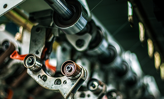 Other tests - pencil hardness test
 Mechanical testing - Packaging compression test
 Climate environment testing - Xenon lamp aging test
Battery Testing
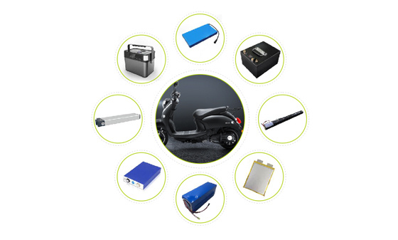 Power storage battery testing and certification
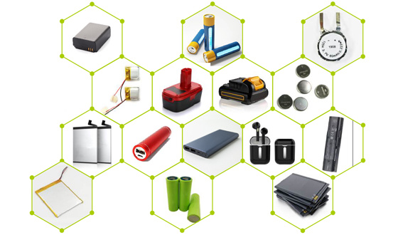 Consumer Electronics Battery Testing and Certification
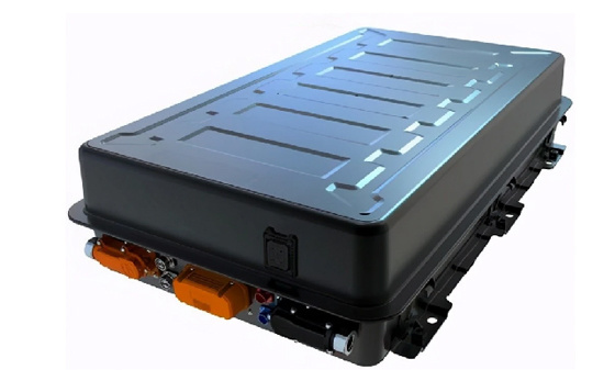 power battery
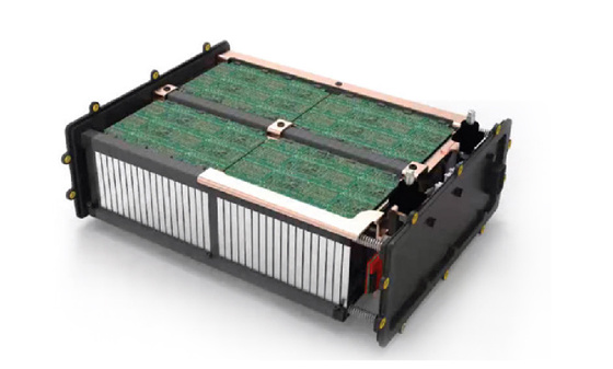 Light electric vehicle batteries
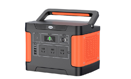 Energy storage battery
 Portable battery
 Battery testing
 battery test
Lamp Inspection
 Inspection of ship lighting fixtures
 COI Index Test for Medical Indoor Lighting
 Lamp safety inspection
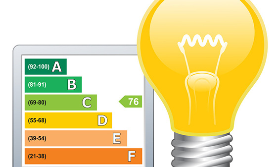 Luminaire energy efficiency testing
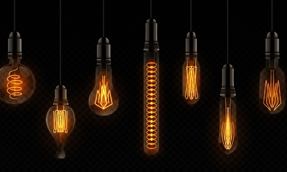 EMC testing of lighting fixtures
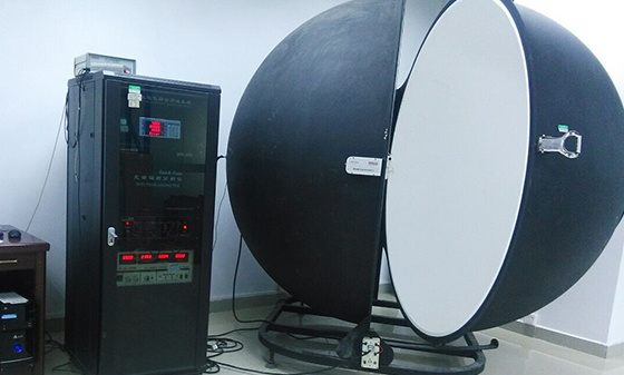 Integral Ball Laboratory
 Photobiology Experiment
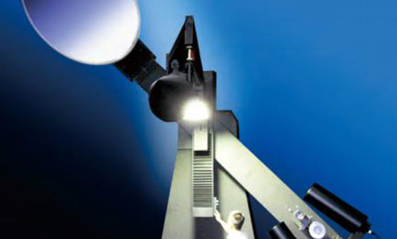 Light distribution test
 Lamp aging test
 Lamp IP waterproof
 Lamp performance testing
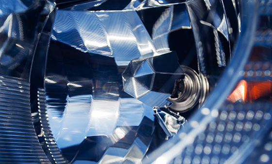 Lamp reliability testing
Children's toy testing
 Testing standards for toy products
China Certification
 China's "national promotion" RoHS certification
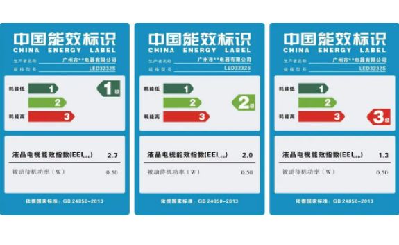 China Energy Efficiency Label Certification
 China Energy Conservation Certification
 China CQC Certification
 Tmall JD Quality Inspection Report
 China SRRC Certification
 Taiwan BSMI certification
 Taiwan NCC certification
 China CCC Compulsory Certification
Asia Certification
 Vietnam certification
 KC certification
 KUCAS Certification in Kuwait
 Singapore PSB certification
 Iraq COC Certification
 IMDA certification
 VCCI Certification in Japan
 JATE certification in Japan
 PSE certification
 BIS certification
 Japanese TELEC certification
European Certification
 RoHS certification
 GOST certification in Russia
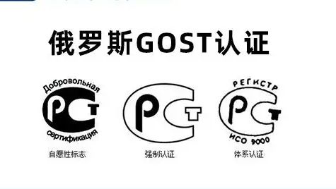 Russian EAC certification
 Northern Ireland UKNI logo
 Electrical ENEC certification
 European D-MARK certification
 Türkiye BTK certification
 TSE certification in Türkiye
 CE certification in Türkiye
 RED certification
 German TUV-SUD certification
 CE-ERP certification
 REACH certification
 German GS certification
 EU E-Mark certification
North American Certification
 Ecuador VOC certification
 Mexico NOM certification
 IRAM certification
 CPSC Certification in the United States
 CSA certification
 ASTM certification
 FDA certification
 CEC certification
 ETL certification
 ul certification
 IC certification
 Energy Star
 FCC Certification in the United States
 ASTM certification
Middle East Certification
 Israel SII certification
 Saudi SABER certification
 GCC certification for the seven Gulf countries
 Iran COI certification
 Qatar COC Certification
 Iraq COC Certification
 Saudi EER Energy Efficiency Certification
 Saudi SABER certification
 Algeria PCA certification
 PVOC certification
Australia Certification
 New Zealand IC-F testing
 VEET certification
 LCP certification
 GEMS certification
 RCM certification
 C-Tick certification
 SAA certification
Africa Certification
 Gabon COC certification
 Algeria COC certification

 Ethiopian VOC and COC certification
 Mauritius VOC certification
 Ghana COC certification
 COC certification in Burundi
 Zambia COC certification
 Botswana COC Certification
 Uganda PVOC certification
 SABS certification in South Africa
 South African LOA certification
 Zimbabwe CBCA Certification
 Nigeria SONCAP certification
 Kenya PVOC certification
 African COC certification
Other certifications
 WEEE
WEEE
 Bluetooth BQB certification
 IECEE registration
 MHRA registration in the UK
TRAINING
 Management system training
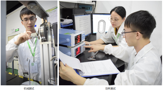 Laboratory technical training
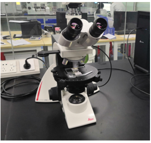 Laboratory Process Consulting
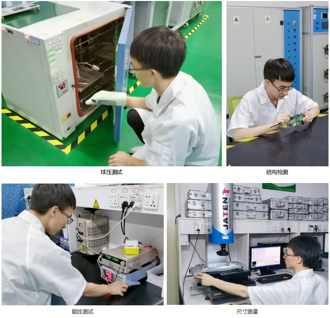 Laboratory decoration construction
Wireless Communication
Electromagnetic compatibility
Automotive Electronics
Automotive Parts Inspection
Electronic appliances
Chemical Testing
Electronic Cigarette Testing
Reliability testing
Battery Testing
Lamp Inspection
Children's toy testing
China Certification
Asia Certification
European Certification
North American Certification
Middle East Certification
Australia Certification
Africa Certification
Other certifications
TRAINING
Wireless Communication
Electromagnetic compatibility
Automotive Electronics
Automotive Parts Inspection
Electronic appliances
Chemical Testing
Electronic Cigarette Testing
Reliability testing
Battery Testing
Lamp Inspection
Children's toy testing
China Certification
Asia Certification
European Certification
North American Certification
Middle East Certification
Australia Certification
Africa Certification
Other certifications
TRAINING
Wireless Communication
Electromagnetic compatibility
Automotive Electronics
Automotive Parts Inspection
Electronic appliances
Chemical Testing
Electronic Cigarette Testing
Reliability testing
Battery Testing
Lamp Inspection
Children's toy testing
China Certification
Asia Certification
European Certification
North American Certification
Middle East Certification
Australia Certification
Africa Certification
Other certifications
TRAINING
Wireless Communication
Electromagnetic compatibility
Automotive Electronics
Automotive Parts Inspection
Electronic appliances
Chemical Testing
Electronic Cigarette Testing
Reliability testing
Battery Testing
Lamp Inspection
Children's toy testing
China Certification
Asia Certification
European Certification
North American Certification
Middle East Certification
Australia Certification
Africa Certification
Other certifications
TRAINING
Wireless Communication
Electromagnetic compatibility
Automotive Electronics
Automotive Parts Inspection
Electronic appliances
Chemical Testing
Electronic Cigarette Testing
Reliability testing
Battery Testing
Lamp Inspection
Children's toy testing
China Certification
Asia Certification
European Certification
North American Certification
Middle East Certification
Australia Certification
Africa Certification
Other certifications
TRAINING
Wireless Communication
Electromagnetic compatibility
Automotive Electronics
Automotive Parts Inspection
Electronic appliances
Chemical Testing
Electronic Cigarette Testing
Reliability testing
Battery Testing
Lamp Inspection
Children's toy testing
China Certification
Asia Certification
European Certification
North American Certification
Middle East Certification
Australia Certification
Africa Certification
Other certifications
TRAINING

Ability Claim | Introduction to MTBF
Author.
LCS
Source:
Post time:
2024-06-25
1、 Definition of MTBF
The full name of MTBF is Mean Time Between Failures. It is a reliability indicator for measuring a product. The unit is "hour". It reflects the time quality of the product and reflects its ability to maintain functionality within a specified time. Specifically, it refers to the average working time between two adjacent faults, also known as the average fault interval. The fewer faults a product has, the higher its reliability. The ratio of the total number of faults in a product to the total number of service life units is called the "Failure rate".
When the lifespan of a product follows an exponential distribution, the reciprocal of its failure rate is called the mean time between failures. That is to say, MTBF=1/λ (where λ is the failure rate)
For example, if a product claims an MTBF of 220000 hours, which is approximately 25 years, it does not mean that the product can work for 25 years without any malfunctions. Because MTBF=1/λ, the failure rate can be calculated as λ=1/MTBF=1/25=4%, which means the average annual failure rate of the product is 4%. That is, within one year, an average of 100 products will have 4 failures.
2、 The purpose of MTBF analysis
Key countermeasures for high-frequency faulty parts and technical transformation basis for extending the service life of parts.
Calculate the lifespan of parts and develop the optimal maintenance plan.
Regarding the selection of inspection objects and projects, as well as the setting and improvement of inspection benchmarks.
Used to guide the allocation of internal and external maintenance work. Based on the evaluation of equipment repair capabilities within the company, the risk of maintenance quality and equipment efficiency is determined by the different types of equipment and job types, which serves as an important reference for maintenance outsourcing.
Set a benchmark for spare parts. The reserve items and basic inventory quantity of mechanical and electrical components should be determined based on the analysis of MTBF records to achieve the most economical inventory level.
As a reference for selecting maintenance techniques and improving key areas. In order to improve the equipment start-up rate, it is necessary to shorten the time for long-term maintenance operations, engineering adjustments, and switching related to equipment shutdown. Therefore, it is necessary to inspect the maintenance operation methods, and the basic information such as the selection of inspection items and priority order needs to be based on the analysis record table of MTBF.
Research on setting estimated running time standards for device objects, as well as selecting maintenance tasks and maintaining time standards. The setting of estimated time standards for maintenance plans and the selection of maintenance tasks must take into account factors such as equipment maintenance repetition cycles or differences between standard time values and actual maintenance time, as well as corresponding maintenance task characteristics. Therefore, an MTBF analysis table is very necessary.
Reference for pattern organization and re selection of key equipment or parts. The analysis record table of MTBF records information on equipment component modification projects or friction degradation, as well as equipment drawing modifications or pre production situations. By regularly conducting analysis and inspection and importance ranking management, engineering drawing management can be made easier.
The setting, revision, and determination of operational standards, as well as the allocation of responsibilities for equipment maintenance business.
Provide technical information on the reliability and maintainability design of equipment. The most important aspect of maintenance technology is to collect technical information on the reliability and maintainability design of equipment based on the MTBF analysis table, in order to provide reference for the design department when designing equipment.
3、 Calculation of MTBF
Assuming a repairable product has experienced N failures during use, and after each failure is repaired, it continues to be put into use for a working time of t1, t2, t3... tN, then the average failure time of the product is T=(t1+t2+t3+...+tN)/N.
Usually, we can see this MTBF value in the product manual or packaging, such as 30000 hours. So, how is the MTBF value calculated? Assuming that the MTBF of a computer is 30000 hours, is it possible to detect it by running it continuously for 30000 hours?
The answer is negative. Currently, there are usually two methods for calculating the MTBF of a product:
1. Traditional reliability prediction methods
Traditional reliability prediction methods are convenient and effective in engineering practice, and have been widely promoted and developed rapidly in various countries. The most commonly used authoritative standards at present are ML-HDBK-217, GJB/Z2998, and Bellcore, which are respectively used for automotive products and civilian products. Among them, MIL-HDBK-217 was proposed by the Reliability Analysis Center of the US Department of Defense and the Rome Laboratory as an industry standard, specifically used for calculating MTBF values of military products; GJB/Z2998 is a military standard in China;
Bellcore was proposed by AT&TBell Laboratories and has become an industry standard for calculating MTBF values for commercial electronic products.
The traditional reliability prediction mainly considers the failure rate of each component in the product, and the failure rate of a product is determined by the various components or modules that make up the product. However, due to the significant differences in failure rates of devices under different environments and usage conditions, for example, the reliability values of the same product will definitely be different in different environments, such as in mainland China and offshore platforms; For example, the failure rate of a capacitor with a rated voltage of 16V is definitely different under actual voltage of 25V and 5V.
Therefore, when calculating reliability indicators, multiple factors mentioned above must be considered. However, these factors mentioned above are almost impossible to calculate manually and must be obtained through software such as MTBFCAL and its vast parameter library.
2. Reliability acceleration model
Life testing is a basic reliability testing method, which is often used to evaluate various reliability characteristics of products under normal working conditions. However, this method is not a suitable approach for products with particularly long lifespans.
Because it requires a long testing time, and even cannot complete the lifespan test in time, new products are designed, and old products are about to be phased out. Therefore, the accelerated life testing method that increases stress and shortens time based on life testing has gradually replaced conventional life testing methods.
Accelerated life testing is a method of increasing test stress (such as thermal stress, electrical stress, mechanical stress, etc.) to stimulate the product to produce the same level of failure as normal stress in a short period of time, shortening the test cycle. Then, using an accelerated life model, evaluate the reliability characteristics of the product under normal working stress. Accelerated environmental testing is a rapidly developing reliability testing technology in recent years. This technology breaks through the traditional approach of reliability testing, introducing the triggered testing mechanism into reliability testing, which can greatly shorten testing time, improve testing efficiency, and reduce testing losses.
The relationship between the lifespan of components and stress is usually based on a certain physical model. Below is a brief introduction to several commonly used physical models.
1) Inefficient model
The inefficiency model divides the failure rate curve into three stages: early failure, random failure, and wear failure, and links the product failure mechanism of each stage with its failure rate to form a bathtub curve. The main application of this model is to eliminate early failed products and improve the reliability of factory products through environmental stress screening tests.
2) Stress and strength model
This model studies the relationship between actual environmental stress and the strength that the product can withstand.
Stress and strength are both random variables, therefore, the failure of a product will depend on the distribution of stress and strength. As time goes by, the strength distribution of the product will gradually change. If stress distribution and strength distribution are intervened, the product will fail. Therefore, studying stress and strength models is important for understanding the environmental adaptability of products.
3) Weakest chain model
The weakest chain model is proposed based on the fact that the failure of a component occurs in the weakest part of the various factors that make up the component.
This model is most effective for studying the failure of electronic products at high temperatures, as such failures are gradually exposed due to potential micro defects and contamination inside the components after manufacturing and use. The most significant and rapid areas of exposure are the weakest and the first to fail.
4) Reaction rate model
This model assumes that the failure of electronic components is caused by physical or chemical changes in the microscopic molecular and atomic structures, leading to degradation in product characteristic parameters. When this degradation exceeds a certain threshold, failure occurs, mainly through models such as the Arrhenius model and the Eyring model.
The environmental factors that determine the lifespan of the entire electrical product are generally temperature and humidity. Laboratories usually use the weakest chain failure model to assess the product's service life by increasing the test temperature and humidity.
Determine the acceleration factor of the product through the Arrhenius model, as well as the Hallberg and Peck models.
The expression for the acceleration factor is:
AF=exp{(Ea/k)*[(1/Tu)-(1/Ts)]+ (RHs^n-RHu^n)}
Among them: Ea: Activation energy (eV, electronic products generally choose 0.65eV)
K: Boltzmann constant, equal to 8.6 * 10-5 ev
T: Absolute temperature (Kelvin temperature)
Tu: The temperature of the product during normal use
Ts: Temperature during acceleration experiment
RHs: humidity during testing
RHs: humidity of the product during normal use
N is the acceleration rate constant of humidity, and different failure types correspond to different values, generally ranging from 2 to 3.
By increasing the testing temperature and humidity, determine the acceleration factor according to the above formula, and calculate the testing time based on the MTBF required by the product.
Related articles
New articles
Media Center
Latest News
Contact Us
National 24-hour service hotline
400-116-2629
Group Headquarters
E-mail: webmaster@lcs-cert.com
Address: Shenzhen City, Baoan District, Shajing Street, Nga side of the school of Wei Juji Industrial Park, Building A 1 ~ 2 floor, Building C 3 floor


 WeChat Inquiry


 Reservation


Contact Us
National 24-hour service hotline
Address:Juji Industrial Park, Xueziwei, Ngabian, Shajing Street, Baoan District, Shenzhen Building A 1~2F, Building C 3F

WeChat public number
Share industry dry goods

WeChat consultation
Please note consulting services

Follow Jitterbug

Mobile website
di complaint mailbox: customer.complaint@lcs-cert.com complaint telephone tel: 18126445450 certificate report verification of authenticity mailbox: verification@lcs-cert.com